
4 Biodiversity Databases
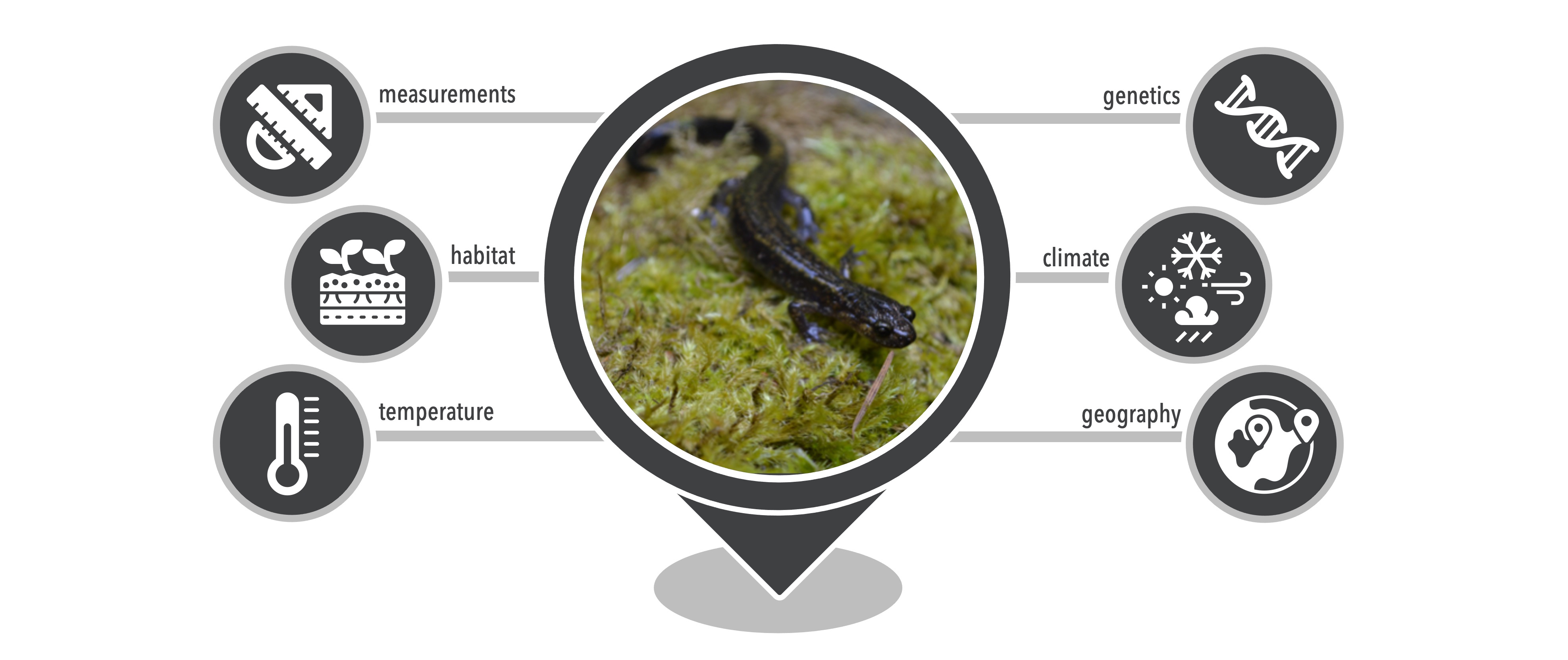
There are many open-source databases that house all types of biodiversity data, and we can use these data to study biodiversity in many different ways. This mostly includes information about what species are found where, but can also include additional information from an individual at a particular location, such as DNA sequence data, sex, body size, or even body condition. These databases are populated by researchers who deposit their data after completion of a research project. For example, researchers have spent many hours in the field searching for several species of Plethodon salamander in the Pacific Northwest of the United States. For every individual they find they record GPS coordinates (latitude and longitude), along with other information about the location and individual. Many researchers also collect a non-invasive tissue sample to sequence DNA for those individuals in order to gain an understanding of the genetic variation within each species. Once finished with a research project, these data are made publicly available by uploading the data to one of many repositories. We will focus on three main data repositories for this book that are used to feed our webserver that creates data-analysis-ready files.
4.1 Global Biodiversity Information Facility (GBIF)
The Global Biodiversity Information Facility GBIF was established in 2001 with the goal to make biodiversity data from specimen collections and observations accessible to anyone anywhere and promote scientific collaboration. It is an international network where members participate in housing computer nodes and making decisions as a collective. As of May 2022, GBIF houses over two billion occurrence records for over one million species, from over 60,000 datasets. While there are geographic biases in the data and not all described species are included (Yesson et al. 2007), this is a massive amount of data! These data have been used to study behavior, systematics, impacts of climate change, invasive species, conservation, and food security issues (see GBIF’s science review for more details).
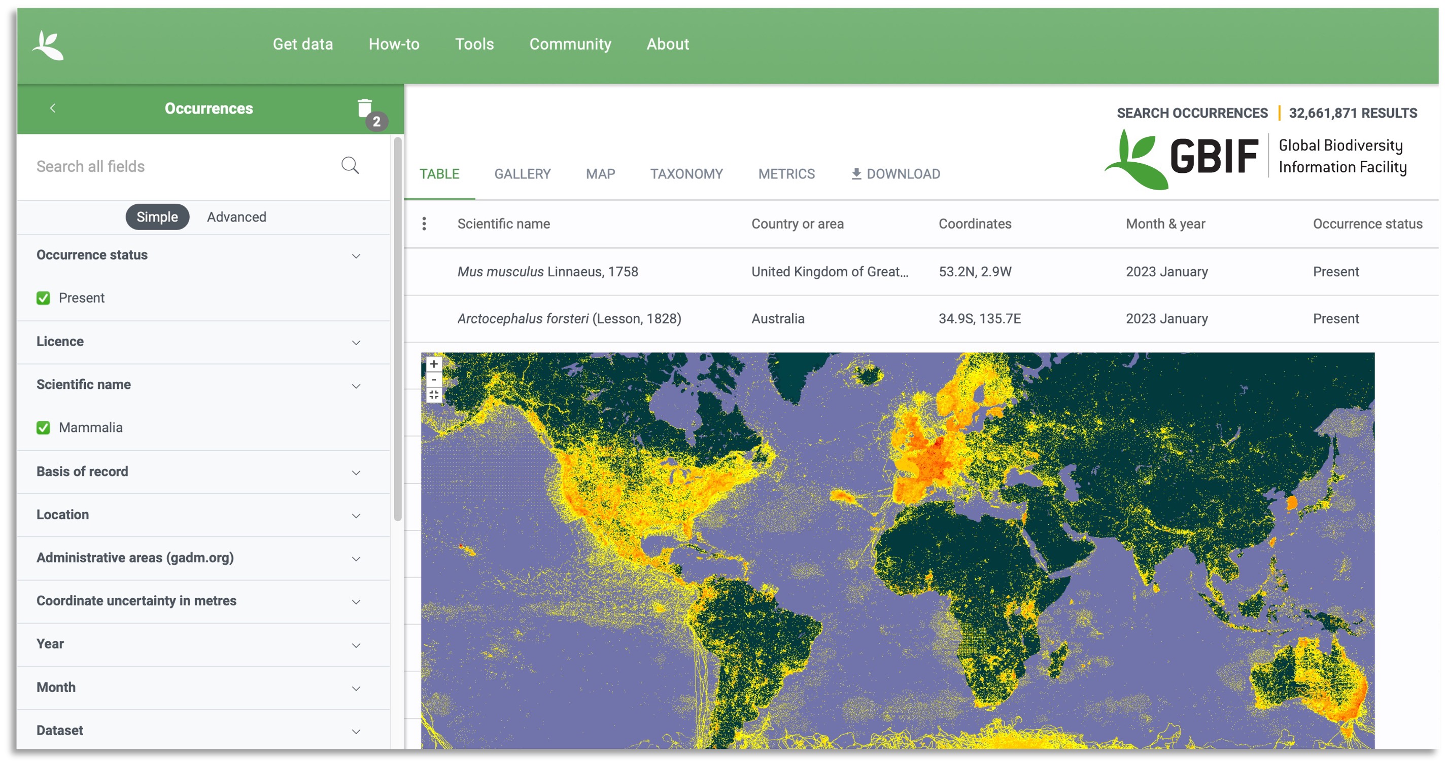
In the example in the opening paragraph, one could supply GBIF with information for each individual salamander for which data was collected. GBIF uses Darwin Core data standards (Wieczorek et al. 2012) and will not accept data that do not comply with these standards. Information from several aspects are required in data submissions, for example, record (e.g., nature of record, observer), event (e.g., date), location (e.g., GPS coordinates, locality descriptions), occurrence (e.g., associated sequence or media data), and taxon (e.g., scientific and common names). Each term has a specific definition in order to standardize the data that is included. When a researcher also generates DNA sequence data associated with the individuals, an identifier for that sequence for that individual that was deposited on a database that houses genetic data can be included.
Some problems that may be encountered when using this database are localities that are in a nearby water body for organisms that are known to be terrestrial, input errors where the sign is reversed for latitude or longitude, or latitude and longitude input as zero rather than identified as missing data. These can be rectified with some data cleaning steps we will discuss later in this chapter.
4.2 GenBank
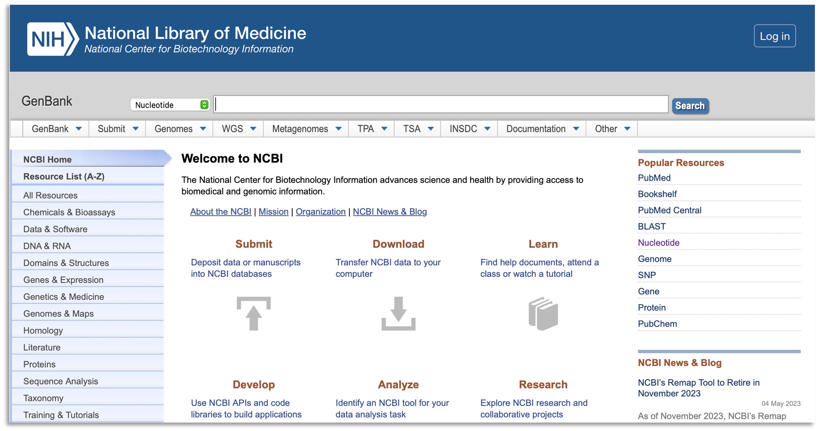
The occurrence data provided by GBIF are used for many purposes in the biodiversity sciences however, associated sequence data from open-source repositories can allow us to ask even more exciting questions in biology! GenBank is a collection of DNA sequence data from three organizations: DNA DataBank of Japan (DDBJ), the European Nucleotide Archive (ENA), and GenBank at NCBI (Benson et al. 2018). The goals of GenBank, released in 1982, are to provide access to and encourage use within the scientific community of the most up-to-date DNA sequence information. There are several ways to obtain these data and several types of DNA data that are stored. We will focus on the Nucleotide database. Once data are submitted and approved, all DNA sequences are assigned a unique identifier called an accession number. GenBank currently houses 218,642,238 sequences and 654,057,069,549 base pairs. Again, this is a massive amount of data!
In the example in the opening paragraph, one would supply GenBank with each DNA sequence for each individual. These data may then be downloaded by other users in conjunction with DNA sequences from other studies and other species to answer all kinds of questions in ecology, evolution, and conservation, many of which we will explore throughout this book.
Some problems that may be encountered when using this database are misidentified species, changes in taxonomy after submission, poorly annotated sequences, and even some sequences that are parasites but are labeled as that species. These issues result in the inability to adequately align DNA sequences for downstream use. There are several steps that can be taken to minimize the amount of messy data, and these will be discussed later in this chapter.
4.3 BOLD
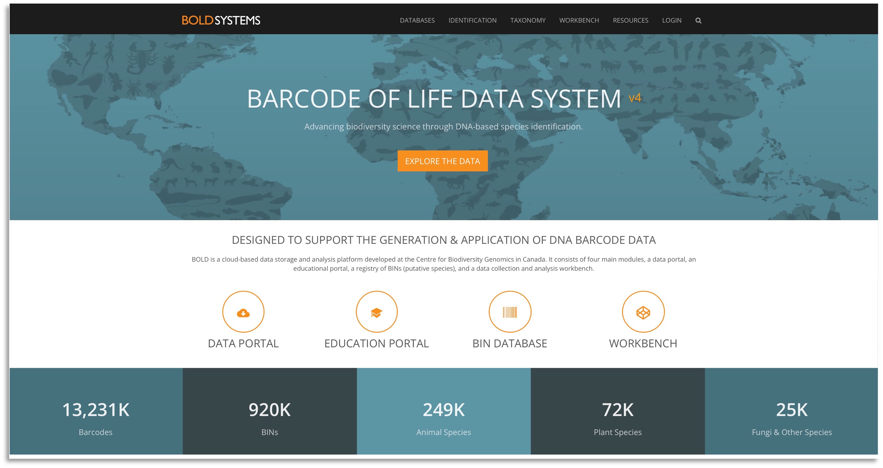
The Biodiversity of Life Database (BOLD) was developed by the Center for Biodiversity Genomics in Canada and contains barcode data for almost 600,000 species from over 1.7 million records. Barcode data are DNA from a specific DNA locus used to identify individuals to species (see Chapter 6). This is often the mitochondrial gene Cytochrome Oxidase I (COI) for animals, the chloroplast genes rubisco large subunit (rbcl) or maturase K (matK) for plants, and the Internal Transcriped Spacer (ITS) for fungi. Data in this portal usually consists of geographic, taxonomic, and natural history collection information. Issues with this database are similar to those described above.
4.4 PhylogatR
Phylogatr (phylogeographic data aggregation and repurposing) links occurrence data from GBIF and sequence data from GenBank so that DNA sequences can be traced to a specific geographic location and analysed in bulk. The data downloads from phylogatr are DNA sequence alignments (as discussed in Chapter 3) with associated GPS coordinates that are analysis ready. Computer scripts are provided throughout this book to assist data analysis and provide user-friendly teaching tools. Analysis of these data can be conducted on the Ohio Supercomputer using R scripts or R Shiny apps provided by the phylogatr team.
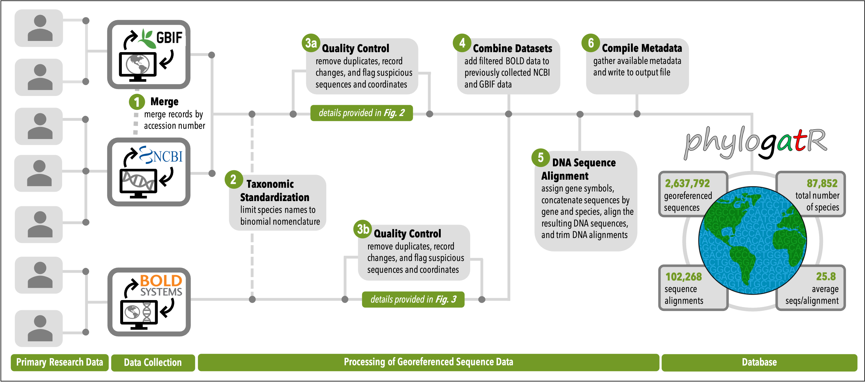 Figure 4E: An overview of the phylogatR pipeline. Figure from Pelletier et al. 2022.
In order to overcome the problems that might be encountered in the databases discussed above, the following data cleaning steps are carried out. Duplicate entries are removed based on a sorting scheme that finds duplicate entries based on the same GenBank number, GBIF identifier, geographic coordinates, species name, and date of occurrence event. Gene names are then standardized to the best of our ability. Mitochondrial gene names were relatively easy to standardize because they are highly represented in GenBank and have an easily manageable number of genes. For example, the cytochrome oxidase b gene might be deposited on GenBank using any of the following abbreviations: Cytb, Cyt-b, COB. These types of issues are problematic for data science projects where we need to group things that are the same and separate things that are different. In this case we can standardize all cytochrome oxidase b sequences by calling them one name: cytb. This is a work in progress and as we learn more about genomics across the diversity of life, we will be able to standardize nuclear gene names more throroughly. Currently, in some instances you might have different gene abbreviations for the same gene across different organisms.
The last step that phylogatr takes is to align sequences that are from the same locus for the same species. We use the program MAFFT v7 to align DNA sequences. During this process sequences are checked that they are going in the same direction. After this step, we need to check the alignments to make sure there are no really short or spurious sequences in the alignment. A bad alignment will vastly overestimate genetic distance among individuals in the alignment (see the last section of this chapter for an example of a bad alignment). We used TrimAI v1.2 to clean up the alignments automatically because there are too many to do this by eye. This step removes sequences that are really short (meaning there is a lot of missing data) so that any downstream analyses are not biased. Then it removes any sequences that do not overlap with the majority of sequences. This allows us to remove DNA sequences that have been labeled incorrectly. For more details on the phylogatr pipeline see the publication and/or GitHub page.
4.5 Using phylogatR
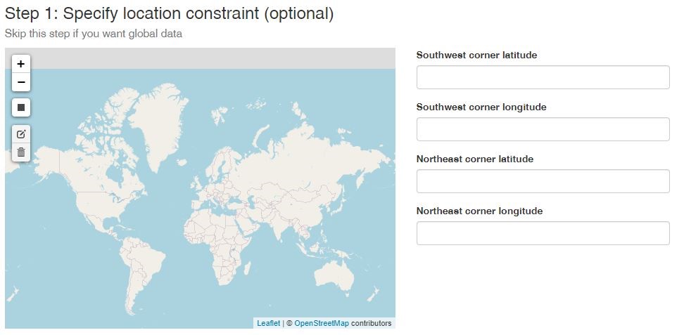
The first step in using phylogatR is to decide what geographic region you are interested in exploring. This can be done by specifying longitude and latitude or drawing a box around the region of interest. Skip this step if you want to download a global dataset. Coming soon: clicking on continents or biogeographic regions
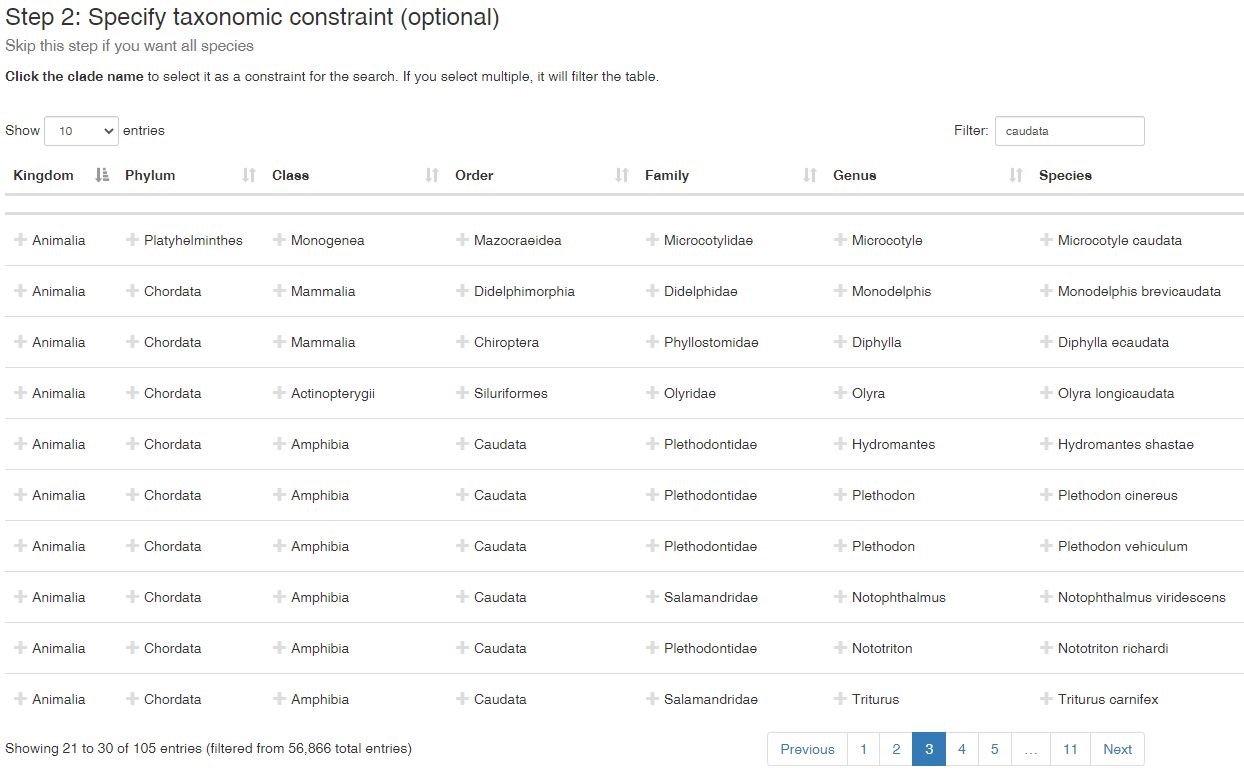
Then identify what taxonomic group you will focus on. In this example, we typed ‘caudata’ (a group of amphibians: salamanders) in the filter box, but you can also click on any names to keep those in your search. If you choose to type in a filter, you’ll want to check the search list because it will retain anything that has ‘caudata’ in the name. For example, see row two below (species: Monodelphis brevicaudata). It is an opossum, but the species name has ‘caudata’ nested within it. I only want salamanders, so I will click on ‘Caudata’ under order so everything else is removed. Skip this step if you want all species available.
The data can be downloaded as a zip file or a tarball, depending on your operating system. Your download will be called phylogatr-results. If you are using a Mac, the zip or tarball file will unzip when you double click on it. If you are using Windows, you must extract the zip file first (this is very important, otherwise the computer won’t recognize the file).The download includes a series of folders that are structured by taxonomy. The root folder will contain two files.
Tab delimited file called
genes.txt. This file contains the gene and species for every alignment in the download, the directory in which the data are found, proportion of sequences retained after cleaning steps, number of unaligned sequences, number of aligned sequences, Kingdom, Phylum, Class, Order, Family, Genus, Species, Subspecies (when applicable), and a column to indicate whether the GBIF and Genbank species names do not match.The
cite.txtfile contains the version numbers used for GBIF, GenBank, BOLD, and phylogatR.
The highest level of taxonomy that will have its own folder is Class. Then a series of folders will be nested within each of these folders, until you get to species. Each species folder will contain the following files:
Fasta file with all the unaligned sequences for each locus with the file extension
.faFasta file with the aligned sequences for each locus with the file extension
.afaTab-delimited file with data for each individual in the sequence alignment called
occurrence.txt. This file contains the GenBank accession, GBIF ID, latitude, longitude, basis of record, geodetic datum, coordinate uncertainty, and identified issues.
4.6 Practice
This module is designed to explore data downloads from phylogatR for observations that look spurious. Data cleaning, and filtering out bad data, is the most important step in a data science project. Bad data = bad results. The code presented here pulls genetic and geographic data downloaded from the phylogatR website and allows you to create a list of sequence alignments that stand out in the data based on estimates of nucleotide diversity. You will then visualize sequence alignments for individual loci simultaneously so that you may check them by eye, and plot geographic coordinates of occurrences on a map for visual inspection.
4.6.0.1 Learning objectives
- Navigate an open-source database.
- Explain why data cleaning is a necessary step in data analysis.
- Quantify outliers from data.
- Identify poorly aligned sequence data.
- Identify geographic outliers.
4.6.1 Downloading data from phylogatR
PhylogatR is a database that supplies users with DNA sequence data from thousands of species that are ready to analyze. There are several steps that needs to be carried out before DNA sequences can be used for data analysis.
- Choose a taxonomic group to assess sequence alignments and geographic coordinates.
- Navigate to the phylogatR website to download data.
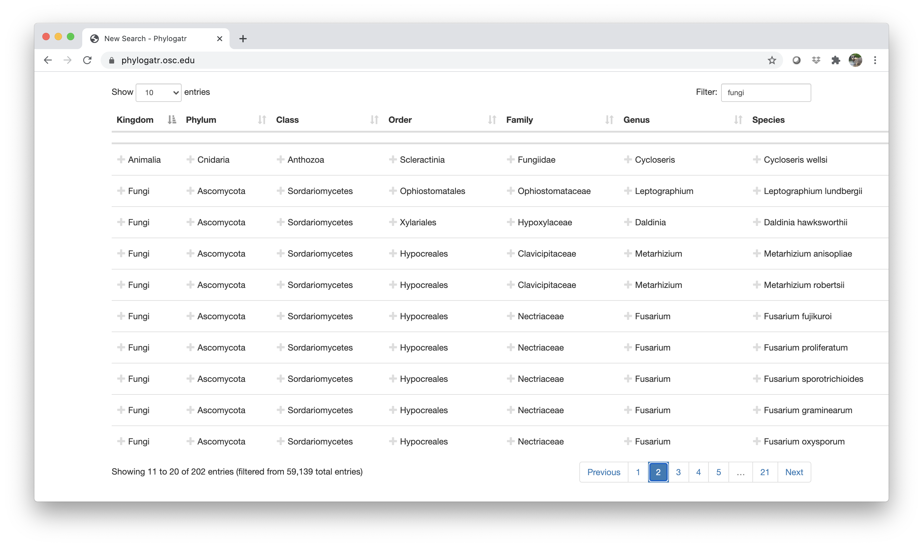
In the example below, fungi was typed into the filter box, but you can also click on any names to keep those in your search. If you choose to type in a filter term, you will want to check the search list because it will retain anything that has fungi in the name. For example, see row two below (Family: Fungiidae). It is a coral, which is an animal, but the Family name has fungi nested within it. If you only want fungi, you will need to click on fungi under Kingdom so everything else is removed. For practice, choose a group that doesn’t contain too many species (<100 species).
Your download will be a zip file called phylogatr-results. If you are using a Mac, the zip file will unzip when you double click on it. If you are using Windows, you must extract the files first (this is very important, otherwise the computer won’t recognize the file).
4.6.2 Check for outliers
This section will take you through the process of estimating nucleotide diversity in a group of closely related species and determine which estimates fall outside of the 95% range of values for this summary statistic.
You will need to load R packages in order to obtain the functions necessary for the analyses that will be conducted. If you have not already installed these packages, you will need to do that first. See here for more information on package installation in R. You will need to install the following packages using the install.packages() function. You only need to install packages once on your computer, but you need to load the library every time you open a new R session.
For example, copy and paste install.packages("tools") into the console in RStudio (bottom left). Do the same thing for each package that needs to be installed for each of the required packages listed below.
- adegenet
- ape
- apex
- ggplot2
- maps
- pegas
- phangorn
- seqinr
- tools
R package issues
If you are still having issues with installing these packages you can use RStudio to update R using the following code. You will need to reinstall any packages that have already been installed before you took this step. For Windows:
install.packages("installr")
library(installr)
updateR()
If you are using a Mac, you can go here and install the newest version on your computer. Restart RStudio and the latest verion of R should be running.
Next, load all the packages necessary for this exercise.
#load necessary packages
library(adegenet)
library(ape)
library(apex)
library(ggplot2)
library(maps)
library(pegas)
library(phangorn)
library(seqinr)
library(tools)
You can ignore messages that might pop up when loading these libraries, unless it is telling you that it is not available, then see above.
4.6.2.1 Explore data
When importing your own data from phylogatR, you will need to change the file path or set your current working directory accordingly. When you import your own data from phylogatR, you might need to change the code below to the correct path. Read more about file paths here.
We are going to explore a small set of mammal data for demonstration purposes. In this case, our current working directory contains the phylogatr-data folder.
Import the genes.txt file to extract information from the download.
genes <- read.delim("phylogatr-results/genes.txt")

nrow(genes)
## [1] 62unique(genes$species)## [1] "Anourosorex squamipes" "Blarina brevicauda"
## [3] "Chimarrogale platycephalus" "Condylura cristata"
## [5] "Crocidura dsinezumi" "Crocidura macmillani"
## [7] "Crocidura olivieri" "Crocidura suaveolens"
## [9] "Crocidura tanakae" "Crocidura wuchihensis"
## [11] "Cryptotis lacertosus" "Cryptotis magna"
## [13] "Cryptotis mam" "Cryptotis merriami"
## [15] "Cryptotis mexicana" "Cryptotis oreoryctes"
## [17] "Neomys fodiens" "Sorex araneus"
## [19] "Sorex arcticus" "Sorex bedfordiae"
## [21] "Sorex caecutiens" "Sorex cinereus"
## [23] "Sorex daphaenodon" "Sorex fumeus"
## [25] "Sorex haydeni" "Sorex hoyi"
## [27] "Sorex isodon" "Sorex longirostris"
## [29] "Sorex minutissimus" "Sorex minutus"
## [31] "Sorex monticolus" "Sorex palustris"
## [33] "Sorex roboratus" "Sorex trowbridgii"
## [35] "Sorex tundrensis" "Sorex vagrans"
## [37] "Sorex volnuchini"Thenrows() function counts how many rows are in your dataset.
4.6.2.2 Import sequence data
First, we are going to create a list of all the sequence alignments and put them in an object called myfiles.
myfiles <- list.files(path = "phylogatr-results", pattern = ".afa", full.names=TRUE, recursive = TRUE)4.6.2.3 Calculate genetic diversity
Here we loop through the list stored in myfiles to calculate genetic diversity for each sequence alignment. All data will be written to a csv file called phylogatr-pi.csv and stored at the path specified at the end of the loop. Here, we are storing the file on my desktop, but you will need to change the path to where you want the file stored accordingly.
for (f in myfiles) {

  #get species and gene name
  sp <- basename(f)
  sp <- file_path_sans_ext(sp)

  #read in fasta file
  seq <- fasta2DNAbin(f, quiet=TRUE)

  #get number of sequences
  n <- nrow(seq)

  #calculate nucleotide diversity
  pi <- nuc.div(seq)


  #write data to file
  write.table(data.frame(sp, pi, n), file="phylogatr-pi.csv", quote=FALSE, row.names=FALSE, col.names=!file.exists("phylogatr-pi.csv"), append=TRUE, sep=",")
}
You will see the error wrong file extension. This can be ignored. It is because we are using .fa and .fas as our file extensions instead of the expected .fasta.
4.6.2.4 Outlier analysis
First, import the output from the previous step. If necessary, change the path to the file accordingly.
data <- read.csv("phylogatr-pi.csv")Print out a list of sequence alignments that fall outside the 95th percentile of the distribution. These may contain poor sequence alignments, though we do recommend checking those that are deemed suspicious by eye. For more information on screening for outliers please see here.
lower_bound <- quantile(data$pi, 0.025, na.rm = T)
lower_bound
## 2.5%
## 0upper_bound <- quantile(data$pi, 0.975, na.rm = T)
upper_bound## 97.5%
## 0.05139108outliers <- which(data$pi < lower_bound | data$pi > upper_bound)
data[outliers,]## sp pi n
## 11 Crocidura-suaveolens-COI 0.08494409 7
## 24 Cryptotis-mexicana-COI 0.05503145 3You might notice that we included a na.rm = T command in the quantile function. This removes any entries that had an NA value as output for the estimate of nucleotide diveristy. Sometimes this happens when something is wrong with the alignment. We can list those here as well to check.
nas <- which(data$pi == NA)
nas
## integer(0)In this case, we did not have any alignments that produced NA values so our object is empty.
4.6.3 Check sequence alignments
We are going to look at the data from the species Sorex monticolus, the Montane shrew, in more detail.
First, we need to store the path names of all of the aligned fasta files for our chosen species. Make sure your path is set to the folder of the species that you want to inspect. We will generate a list of paths to all of the aligned fasta files (i.e., all files in the species folder that end in .afa) using the function list.files and store this list in R as myfiles. This is similar to what we did above, but we are listing those from a different folder. Notice that we have overwritten the myfiles R object with with a new list.
#get paths to aligned fasta files in species folder (all .afa files in downloaded phylogatR folder)
myfiles<-list.files(path="phylogatr-results/Mammalia/Soricomorpha/Soricidae/Sorex-monticolus", pattern=".afa", full.names=TRUE)
Next, we will use the paths stored in myfiles to import our aligned fasta files and create a multidna object. A multidna object is a class of object used to store multiple DNA sequence alignments. Sequences are stored as a list, with each element of the list being a separate DNA alignment stored as a DNAbin matrix. For more information on DNAbin and multidna objects, see here.
We will use the function read.multiFASTA to create a multidna object containing our aligned fasta files. In the likely case that some individuals are not sequenced for all loci, setting the argument add.gaps to FALSE will ensure that indivuals that do not have a sequence for a locus (gap only sequences) will not be added to the alignment.
#create S4 class multidna object (contains DNAbin objects for all loci/.afa alignment files)
multidna<-read.multiFASTA(files=myfiles, add.gaps=FALSE)
Now we will use the plot function to visualize the separate alignments (i.e., loci) in our multidna object simultaneously. When set to FALSE, the argument rows will return each locus in a separate image. If set to true, all loci will be shown in a single image (note: depending on how many alignments you have, setting rows=TRUE may make your alignments too small to inspect).
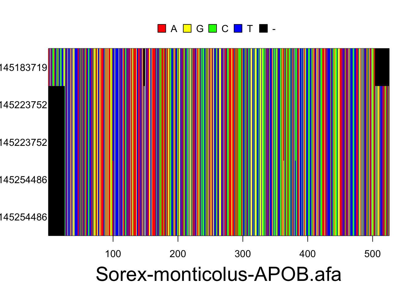
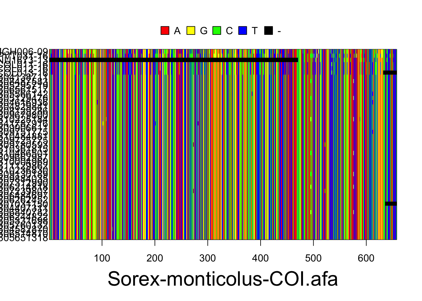
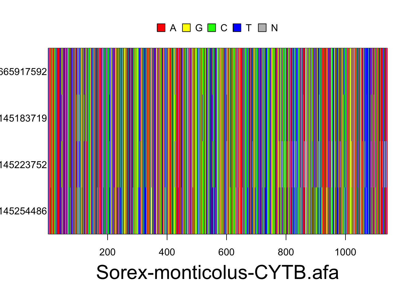
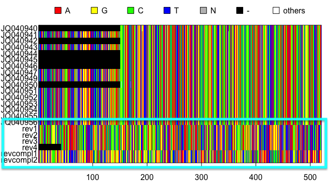
The resulting alignments will consist of a series of rows (each representing the DNA sequence of one individual) and columns (each representing a particular nucleotide position in the locus). Accession numbers for each individual are located to the left of each row and the species and gene/locus name are located at the bottom of the alignment. Nucleotides are color coded according to the legend located at the top of the alignment. These plots are for the Sorex monticolus data. Your plots should look something like this.
#visualize the separate alignments in your multidna object simultaneously
plot(multidna, rows=FALSE, ask=FALSE)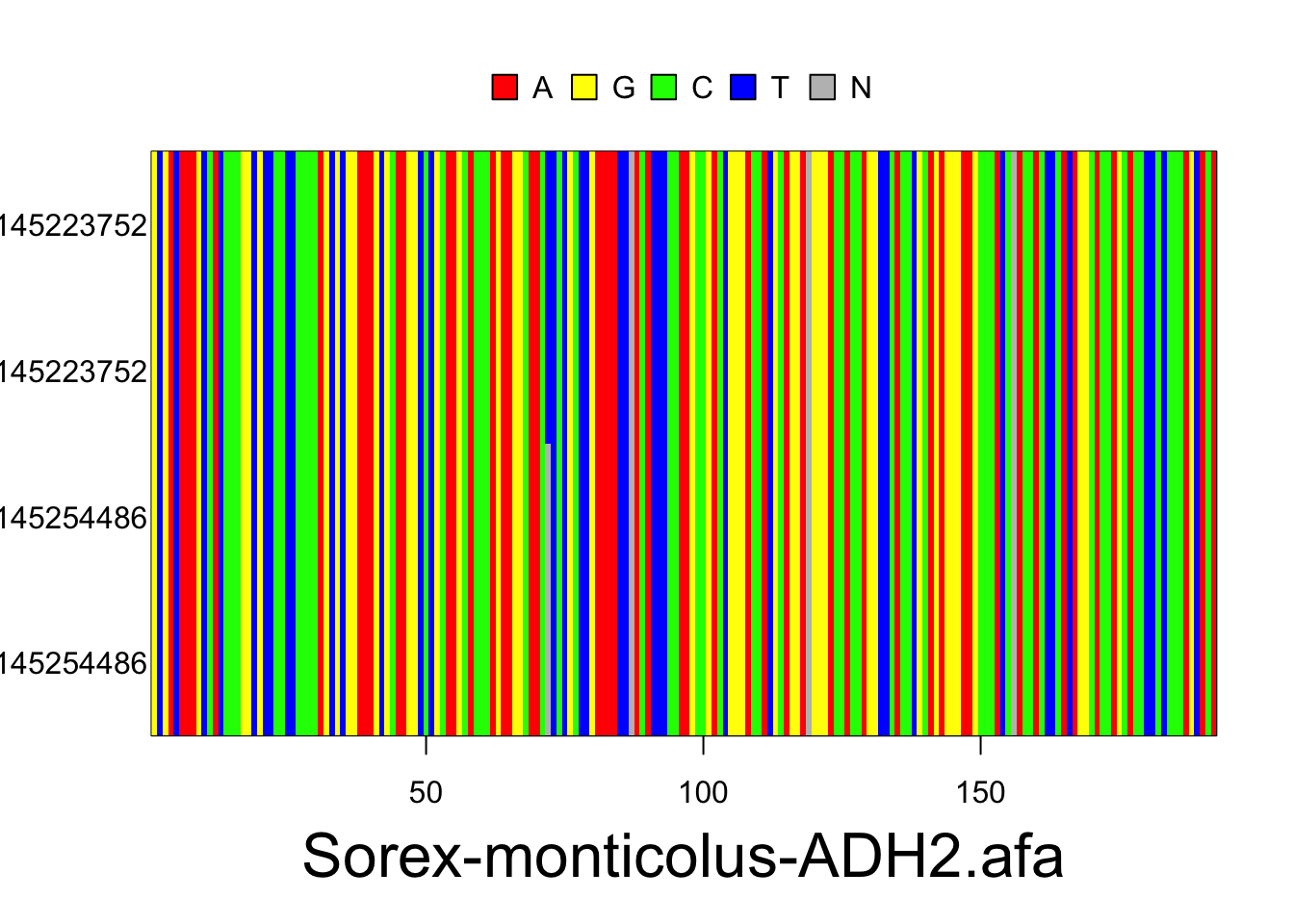
Use the following code to export your alignments as a pdf. They will be exported as sequences.pdf into your current working directory, unless you change the file path.
#export sequence alignments
pdf(file="sequences.pdf")
plot(multidna, rows=FALSE, ask=FALSE)
dev.off()
Sequence alignments: what to watch out for
The following alignments are meant to show you potential errors you might run into when inspecting your sequence alignments. PhylogatR takes steps to minimize these issues (see here), but it never hurts to check your data.
In the first example, we have edited the alignment to contain sequences that have been entered in reverse (rev1-4) and reverse complement (revcompl1-2). As you can see, these sequences are comparable in length to the rest of the alignment and are lacking large regions of gaps. However, upon visual inspection they clearly do not line up with the rest of the alignment. These sequences can be checked and edited manually in a sequence viewing program (e.g., UGENE or mesquite).
In this example, we have added parasitic sequences (parasite1-3) to the alignment. These sequences contain long regions of gaps and the regions of nucleotides present do not line up with the rest of the alignment. If your alignment has questionable sequences such as these, you can do a search of their accession numbers here to ensure they are from the correct species and locus.
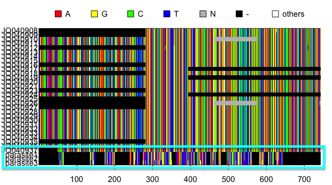
If needed, you can submit corrections to GenBank sequence data by sending an error report to update@ncbi.nlm.nih.gov.
4.6.4 Visualizing geographic coordinates
Now we will use the occurrences.txt file located in the species folder of our phylogatR download to plot geographic coordinates for all individuals within our species folder and check for potential errors. First, we will import our occurrences.txt file, found in our species folder, into R and save it as a data frame called occurrences.
Once that data file has been imported into R, we will extract just the columns containing latitude and longitude (i.e., columns 4 and 5) and save them in R as an object geo.
#read in geographic coordinates
occurrences<-as.data.frame(read.table("phylogatr-results/Mammalia/Soricomorpha/Soricidae/Sorex-monticolus/occurrences.txt", header=TRUE, sep="\t"))
#extract latitude and longitude
geo<-occurrences[,c(4:5)]
Now we will plot our geographic coordinates on a map to inspect for errors. In the resulting map, each red dot represents a single sampling locality. Please keep in mind that when using geographic coordinates in R, longitude (the x-axis) comes first, and latitude (the y-axis) comes second.
#plot localities
world<-map_data("world")
ggplot()+
  geom_polygon(data = world, aes(x=long, y = lat, group = group), fill = "lightgrey", color = "gray30", size = .25)+
  coord_fixed(1.3)+
  xlab("Longitude")+
  ylab("Latitude")+
  ggtitle("Collection Locality Geographic Coordinates")+
  geom_point(data = geo, aes(x = as.numeric(geo$longitude), y = as.numeric(geo$latitude)), color = "red", size = 0.8)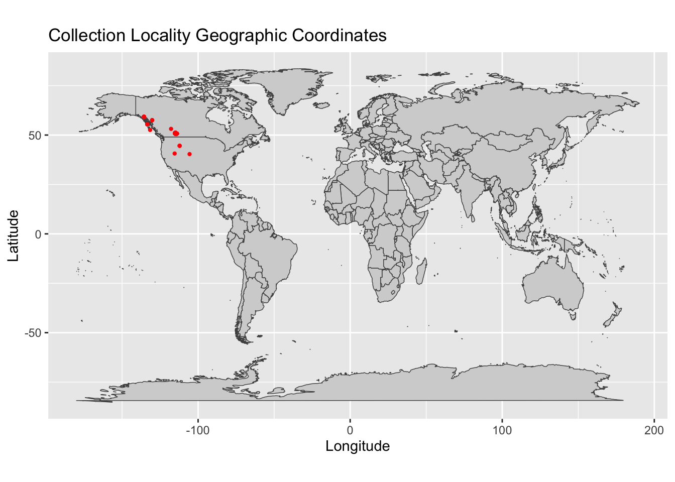
Geographic coordinates: what to watch out for
The following map is meant to show you potential errors you might encounter when inspecting your geographic data. You’ll want to look out for any data points that are obviously outside of your species expected range. Data points that are very far away from the rest of the points (i.e., outliers) as well as data points in areas physiologically unlikely for your species (e.g., a terrestrial shrew in the middle of the ocean) should warrant further inspection. If you are unsure of the extent of your species range, you can search for your species here.
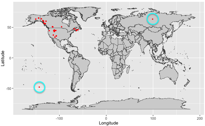
If needed, you can submit corrections to GBIF occurrence data by clicking the speech bubble icon in the upper right corner of the GBIF website.
To summarize, it is always a good idea to check your data before you begin your data analysis steps. The phylogatR teacher resources page has additional R code that explores these issues in more detail.